Transient Analysis Friction Methods

Steady Friction

In HAMMER, a hydraulic transient analysis usually begins with an Initial Conditions (steady state) calculation, which computes the heads and flows for every pipe in the system. Prior to beginning the transient calculations, HAMMER automatically determines the friction factor based on this information:

If a pipe has zero flow at the initial steady-state, HAMMER uses the Friction Coefficient specified in the Pipe Physical properties. (Alternatively, if the user has the 'Specify Initial Condition' Transient Solver calculation option to True, the user must enter a Darcy-Weisbach friction factor, f)
If a pipe has a nonzero flow at the initial steady-state, HAMMER automatically calculates a Darcy-Weisbach friction factor, f, based on the heads at each end of the pipe, the pipe length and diameter, and the flow in the pipe. It uses this calculated value in the transient simulation.

Note: HAMMER always uses the Darcy-Weisbach friction method in performing the hydraulic transient calculations, regardless of which method is specified in the Steady State/EPS Solver Calculation Options. If required, HAMMER will automatically convert user-entered friction factors to the appropriate format.

Distributed frictional losses are assumed to be concentrated at discrete computational points treated as hypothetical inline orifices. The head difference between the upstream and downstream side of the orifice is typically taken to be proportional to the square of the instantaneous velocity as in the Darcy-Weisbach equation.

Consequently, at every calculation point, there are two heads: one on the upstream side and one on the downstream side as indicated in the figure below (Bergeron, 1961). These differ by the head loss between adjacent calculation points. The addition of the nonlinear equation Darcy-Weisbach equation to the system of characteristic equations does complicate the task of advancing the solution forward in time, and leads to an approximation in terms of the friction coefficient which is typically small.

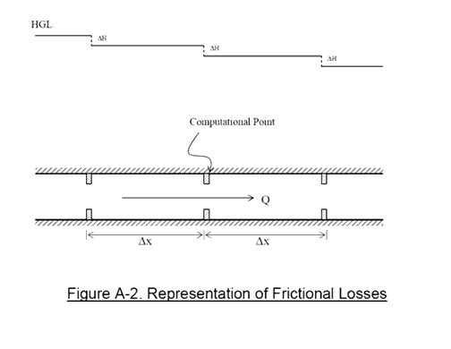
Historically (Parmakian, 1961; Wylie and Streeter, 1993), in simulating unsteady flow in closed conduits, frictional losses have been represented by means of a steady-state friction coefficient as derived from the initial conditions and/or the entered value in the case of zero-flow pipes. For each artificial inline orifice, a head-loss coefficient is determined so that the total pipe loss due to the summation of such local losses is identical to the distributed loss of the pipe. After the coefficients are calculated initially, they remain invariant throughout the run.